KIAS — AI and Maths 2026
Gauge theories · AI for Physics · Physics for AI
AI for Mathematics (Physics) · Mathematics (Physics) for AI
Three fields of research (and more...)
Dimer models and toric Calabi–Yau
Dimer models and toric Calabi–Yau
Neural networks on dimer models
 P. Capuozzo
 T. Schettini
Gherardini
T. Schettini
Gherardini
Question: what hidden structure can ML help us identify?
→ unsupervised learning, explainable AI, …
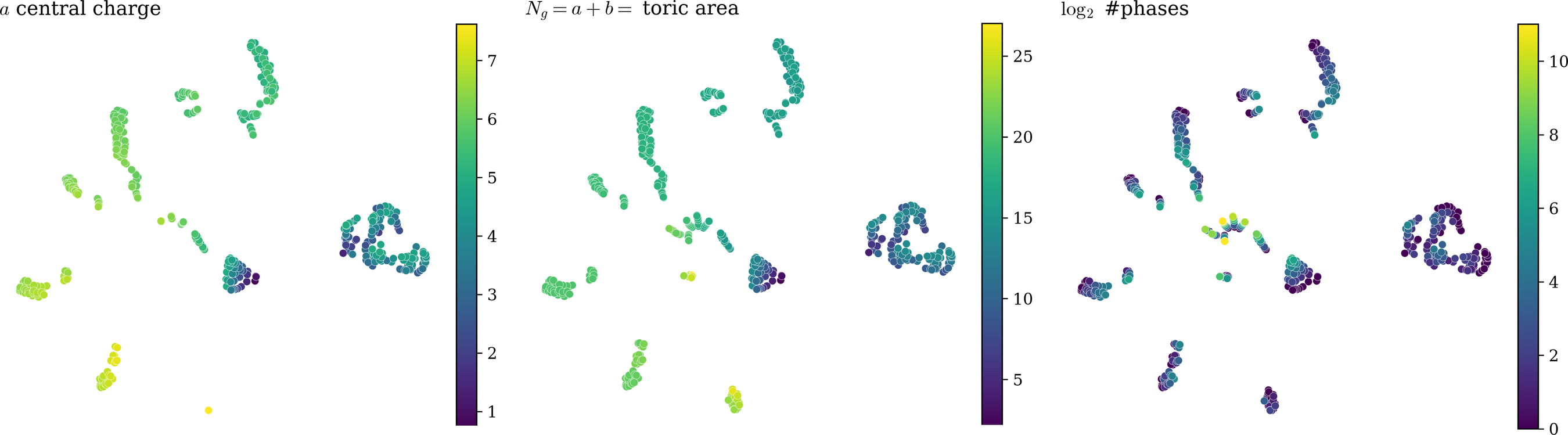
label-free embedding, coloured by physics it was never shown
The Neural-Network Field-Theory correspondence
The textbook description of a QFT is the path integral
\[ \langle\mathcal{O}(x)\rangle = \int\mathcal{D}\phi\; e^{-S[\phi]}\, \mathcal{O}(x) \]
but the measure \(\mathcal{D}\phi\) is generally not well defined — it is shorthand for "integrate over all fields".
We can define it
- rigorously, sometimes (e.g. TQFTs)
- by discretizing space (lattice)
- or with neural networks and UATs
Key idea: use the initialization distribution together with the UAT to integrate over all network configurations.
\[ \int\mathcal{D}\phi\; e^{-S[\phi]}\,\mathcal{O}(\phi(x)) \qquad\longleftrightarrow\qquad \lim_{N\to\infty}\int_{\Omega}\prod_i^N d\theta_i\, P(\theta_i)\,\mathcal{O}(\phi_\theta(x)) \]
Correlators — and interactions
Correlators come from the generating functional, now an ordinary expectation value:
\[ Z[J] = \lim_{N\to\infty}\int_{\Omega}\prod_i^N d\theta_i\, P(\theta_i)\; e^{\int dx\, J\phi_\theta} \] \[ \frac{\delta^2 Z[J]}{\delta J(x)\delta J(y)} = \mathbb{E}_{P(\theta)}\big[\phi_\theta(x)\phi_\theta(y)\big] = K(x,y) \]
A free scalar with propagator \(K\):
\[ S[\phi] = -\frac{1}{2}\int dx\,dy\; \phi(x)\, K^{-1}(x,y)\, \phi(y) \]
Two ways to switch on interactions:
Finite-\(N\) corrections
step back from the UAT limit
Break the UAT requirements
e.g. statistical dependence of the parameters
e.g. \(\phi^4\)-theory, as a deformation of \(P(\theta)\):
\[ P(\theta) \;\longrightarrow\; P(\theta)\, \exp\left(-\frac{\lambda}{4!}\int dx\; \phi_\theta^4(x)\right) \]
Choosing \(P(\theta)\) and \(\phi_\theta\) — hence \(K\) — engineers different QFTs; leaving the UAT limit switches on the interactions.
Where the field is heading
- Recover known theories — gauge theories, supersymmetric strings, CFTs — as architectures
- Rederive their known predictions, now with the tools of NN-FT
- Predict new results inside those same theories
- Discover new theories, and their properties
- Flow the distribution \(P(\theta)\) (is learning an RG flow?)
One of the goals: use the tools of QFT to study general ML setups: Physics for AI
 C. Ferko
 S. Frank
 J. Halverson
 V. Jejjala
 B. Robinson